Keynote speech by Philip R. Lane, Member of the Executive Board of the ECB, at the Bank of England Watchers’ Conference 2024, King’s College London
London, 25 November 2024
Introduction
My aim today is to explain how uncertainty is incorporated in the monetary policy process at the ECB.[1][2] While monetary policy makers have always had to grapple with uncertainty, recent years have been marked by a pronounced increase in the quantum of uncertainty. This includes the uncertainties related to the pandemic and the unjustified Russian invasion of Ukraine (Chart 1). It also includes the uncertainties related to technological change, geo-economic trends and the green transition.[3] In this speech, I will discuss how the ECB incorporates risk and uncertainty in its forecasting, in the preparation of monetary policy decisions and in communication.[4]
Chart 1
Macroeconomic uncertainty, forecast disagreement, economic policy uncertainty and VSTOXX
(left scale: macroeconomic uncertainty, forecast disagreement and economic policy uncertainty, all standardised indices; right scale: VSTOXX, index)
Sources: Jurado et al. for macroeconomic uncertainty, Consensus Forecast and ECB calculations for forecast disagreement, Baker et al. for economic policy uncertainty, LSEG, Bloomberg, and ECB calculations for VSTOXX. Notes: The chart shows the monthly average for VSTOXX. The latest observations are for September 2024 for macroeconomic uncertainty and October 2024 for the rest. Jurado et al. refers to Jurado, K., Ludvigson, S.C., and Ng, S. (2015), “Measuring Macroeconomic Uncertainty”, American Economic Review, Vol. 105, No. 3, pp. 1177-1216. Baker et al. refers to Baker, S.R., Bloom, N., and Davis, S.J. (2016), “Measuring Economic Policy Uncertainty”, Quarterly Journal of Economics, Vol. 131, No. 4, pp. 1593-1636.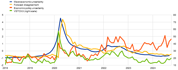
Events such as the global financial crisis, the pandemic and wars are inherently unpredictable. And, even once such an event has occurred, its ultimate impact on the economy is very difficult to work out. A prime example is Russia’s invasion of Ukraine. By triggering extraordinary jumps in gas and oil prices, and by creating a generalised sense of insecurity, this conflict was a major driver of the recent surge in inflation and also brought geo-political risk considerations to the fore. The scale and duration of the conflict have had wider ramifications for the euro area economy, also prompting difficult questions about the appropriate scale of defence spending and the management of the economic and social impact of refugee flows.
One “uncertainty tracker” is the risk index developed by ECB staff based on importance of the different risks articulated in the earnings calls of publicly-traded euro area companies (Chart 2). While this summary indicator shows some decline in risk intensity recently, primarily due to a decline in uncertainty related to macroeconomic developments and supply chain disruptions, it remains above pre-pandemic levels.[5]
Chart 2
Risk index
(percentage of all risk sentences)
Sources: NL Analytics and ECB calculations . Notes: The series are based on textual analysis of earnings calls for euro area firms up to the third quarter of 2024 for a number of macro risks, reflecting searches for words associated with the respective risks. See Andersson, M., Guillotin, J. and Neves, P. (2024), “Insights from earnings calls – what can we learn from corporate risk perceptions and sentiment?”, Economic Bulletin, Issue 4, ECB.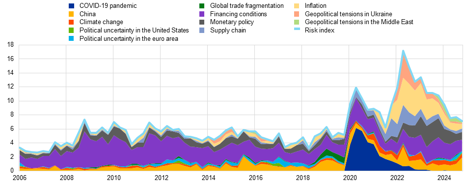
Yet even in quieter periods not featuring extraordinary events, uncertainty is an inherent aspect of decision making in economics. The fundamental unpredictability of the future creates a cone of multiple possible outcomes, each with its own set of implications. Uncertainty may also stem from environments that cannot be observed or characterised in their entirety when incomplete information adds another layer of unpredictability.
There is a long history to the challenge of incorporating uncertainty into economic decision making. Economists and policymakers have long recognised that the economy is subject to shocks and that human behaviour, which underpins economic activity and shapes collective reactions to the shocks, is inherently unpredictable.
Some economists have argued that individuals and markets can, on average, formulate an accurate risk distribution over future events by using all available information.[6] In this way, uncertainty can be captured in standard macroeconomic models by the use of probability distributions around different outcomes or scenarios, which can either be measured directly or estimated (for example, from financial options markets). Even when risks can be measured and quantified, the way in which this affects economic decisions may be highly complex and non-linear, as emphasised by complexity theory.[7]
In this context, it can be useful to distinguish between what is often called ‘risk’ – which can be modelled via known calculable probabilities – and Knightian uncertainty, where there is no objective basis for deriving probabilities and one may not even be able to delineate the space of all the circumstances that can occur. Under this Knightian form of uncertainty, risks are not known or even knowable, making them impossible to quantify and forecast. This distinction has its foundations in seminal works by Frank Knight and John Maynard Keynes.[8]
Decision-making under this type of uncertainty may not be well captured by our standard models. For example, developments in behavioural economics have shown that cognitive biases can significantly affect decision-making under uncertainty.[9] Other strands of research have demonstrated that relying on simple heuristics can be a boundedly-rational response in complex environments.[10] Under this type of uncertainty, the development of scenarios and application of judgment about possible outcomes in the future can complement models and help policymakers adjust and adapt policy action when needed.
These considerations highlight the importance of practitioners taking a nuanced approach towards risk management. A comprehensive approach calls for the adoption of robust strategies consistent with a wide range of risk scenarios. In addition, policy should acknowledge the limits of predictability and follow an adaptive approach, leaving enough room for manoeuvre when faced with genuine surprises.[11]
With this in mind, I will use the remainder of my time to explain the broad range of strategies that are used at the ECB to quantify and incorporate risk and uncertainty into macroeconomic forecasting and in making monetary policy decisions. I will also discuss how risk and uncertainty are articulated in the monetary policy communication of the ECB.
Uncertainty about the economy and monetary transmission
The inflation surges in the euro area during 2021 and 2022 resulted from a sequence of large shocks, which also precipitated a significant burst of uncertainty. These shocks related both to the longer-term fallout from the pandemic and the Russian invasion of Ukraine, with demand rotating across sectors in an environment in which some key segments of the economy were supply constrained. In addition, the war-induced subsequent surges in energy prices infiltrated the entire price chain.
Macroeconomic projections are a key input to forward-looking monetary policy decision making. But forecasting models – which embed economic relations based on historical regularities and typically struggle to handle pervasive uncertainty – naturally faced significant challenges during this period. From the middle of 2021 to early 2023, this challenge was visible in the scale of realised forecast errors for both headline and core inflation, as well as real GDP growth (Chart 3). During this period, the significant forecast inaccuracies were driven by pandemic-related bottlenecks and the dramatic surges in energy and commodity prices. But shifts in how these shocks were transmitted to inflation, including owing partly to pandemic reopening effects, also played an important role in the broadening of the inflation shock, increasing its size and persistence.[12]
Chart 3
One-quarter-ahead errors in the inflation projections of Eurosystem/ECB staff
|
HICP inflation |
HICPX inflation |
Real GDP growth |
|---|---|---|
|
(annual percentage changes) |
(annual percentage changes) |
(annual percentage changes) |
 |
 |
 |
Sources: Eurostat and Eurosystem/ECB staff macroeconomic projections for the euro area.
Notes: An error is defined as the outturn for a given quarter minus the projection made for that quarter in the previous quarter (for example, the outturn for the fourth quarter of 2022 minus the figure projected for that quarter in the September 2022 ECB staff macroeconomic projections). The latest observations are for the September 2024 ECB staff macroeconomic projections.
Faced with these major events that challenged our existing processes, models and forecasts, the ECB has developed strategies to support decision-making in managing and mitigating uncertainty. I turn to these strategies in the next section.
The three-pronged reaction function
In general, central banks make monetary policy decisions on the basis of two factors: first, the “most likely” (or baseline) projection for inflation and output; and, second, the risk profile surrounding this expected path. In guiding the disinflation process since the inflation peak in late 2022, the most prominent risks facing the ECB were: (i) in the context of extraordinarily-high inflation, there was a wide distribution of possible inflation paths, such that the weight attached to the baseline projection in updating beliefs about inflation dynamics was naturally lower than normal, with a corresponding step up in the attention paid to the realised path of underlying inflation; and (ii) in the context of a steep rate hiking cycle (especially after an extended low-for-long monetary environment), there was considerable uncertainty about the strength of monetary policy transmission. These risks were best managed by adopting a three-pronged reaction function encompassing both information from staff projections and cross-checking information from a variety of sources. Since March 2023, the Governing Council has communicated that it is particularly attentive to: (i) the implications of the incoming economic and financial data for the inflation outlook; (ii) the dynamics of underlying inflation; and (iii) the strength of monetary policy transmission.[13]
This strategy has proved its value in ensuring an orderly disinflation process by setting the interest rate path to deliver a timely return of inflation to the target. In particular, by systematically considering all three elements of the reaction function and weighting them appropriately, the Governing Council could better calibrate monetary policy in the face of unpredictable, sometimes contradictory information.[14] This three-pronged reaction function can be understood as a heuristic for simultaneously managing multiple sources of uncertainty during the disinflation process, both in relation to inflation dynamics and the transmission of monetary policy.[15]
The inflation outlook
The first element of the reaction function is the inflation outlook, which can be understood to encompass both the “most likely” future path for inflation and the surrounding risk assessment. The assessment of the inflation outlook is based on the incoming economic and financial data. The quarterly staff macroeconomic projection exercise is a central input into this assessment, as it aggregates a vast amount of information that would otherwise be hard to map into a coherent profile of the future path for inflation and output. At the “in between” non-projection meetings, the incoming information is best interpreted through the lens of the latest projection round, either validating or casting doubt on these projections. In synthesis, our assessment evolves according to a Bayesian-style updating process, with priors at inter-projection meetings pinned down by the latest projections and incoming statistics helping to update the picture. Chart 4 shows the path of inflation as foreseen in the September staff projections.
Chart 4
Euro area HICP inflation: data and baseline forecast
(annual percentage changes)
Sources: ECB calculations. Notes: The vertical line indicates the start of the current projection horizon. Inflation before this vertical line indicates data. The horizontal line indicates the 2% inflation target.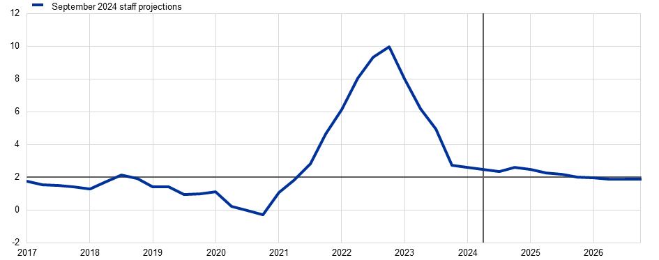
Underlying inflation
Measures of underlying inflation provide a useful alternative perspective in assessing inflation dynamics, especially in times of elevated uncertainty.[16] Measures of underlying inflation aim to filter out the short-term volatility in headline inflation to better capture the low-frequency component of inflation. Accordingly, such measures provide a sense of where headline inflation is likely to settle in the medium term, once temporary factors have dissipated.
Unlike headline inflation, many measures of underlying inflation are not directly observable and must be estimated. In times of uncertainty, examining a range of measures of underlying inflation is particularly important, since no single measure is a perfect proxy for medium-term inflation trends. Such an approach ensures that no individual measure is over-emphasised as being higher or lower in any given period. The range across different measures of underlying inflation also provides an indication of the level of uncertainty, as can be seen from the wide range during 2022 and 2023 and its recent narrowing (Chart 5).
At the same time, the major economic disruptions of recent years also meant that the standard set of underlying inflation measures became less informative for medium-term inflation developments. In particular, the bottleneck and energy shocks exerted a significant persistent-but-not-permanent impact on such measures, such that the standard measures likely over-stated the scale of the increase in the underlying inflation component.
Accordingly, ECB staff also developed complementary “adjusted’’ measures of underlying inflation that filtered out the exceptional influences from supply chain bottlenecks and energy price shocks in the post-pandemic recovery.[17] When adjusting for these shocks, the peak of underlying inflation measures was lower and the range was narrower during the high inflation period (Chart 5). With the fading of the bottleneck and energy shocks, the gap between the adjusted and standard measures of underlying inflation has declined.
Chart 5
Range of underlying inflation measures and measures adjusted for the impact of supply bottleneck and energy shocks
(annual percentage growth)

Sources: Eurostat and ECB staff calculations.
Notes: Range of underlying inflation measures include: HICP excluding energy, HICP excluding unprocessed food and energy, HICP excluding energy and food (HICPX), HICP excluding energy, food, travel-related items and clothing (HICPXX), PCCI, PCCI excluding energy, Supercore and domestic inflation. The “adjusted” measures abstract from energy and supply bottleneck shocks using a large SVAR (see Bańbura, M., Bobeica, E. and Martínez Hernández, C. (2023), “What drives core inflation? The role of supply shocks”, Working Paper Series, No 2875, ECB), subtracted mechanically from each measure. The latest observations are for September 2024.
Monetary policy transmission
The third element of our reaction function seeks to capture the inherent uncertainty in how monetary policy is transmitted to financing conditions, the broader economy, and ultimately inflation. The reason for these uncertainties – explicitly recognised in the 2021 monetary policy strategy statement, which emphasises the “lags and uncertainty in the transmission of monetary policy to the economy and to inflation” – lies in the ever-evolving nature of financial intermediation. Together with the scale of the shocks hitting the economy and the speed and scale of the monetary policy tightening cycle, the state-contingent responses of banks and other intermediaries influence how strongly policies are transmitted to the broad economy.
At the start of the tightening cycle, it was not obvious how forcefully increases in the key policy rates would be transmitted along the yield curve and to broader financing conditions.[18] That is why, in accordance with the data-dependent approach, it was important to carefully check the evolution of bank funding costs, borrowing costs for households and firms, and credit growth. These statistics (which arrive only with a lag) were complemented with additional insights from other sources. These include the bank lending survey (BLS), which captures changes in credit standards and credit demand from households and businesses, and the survey on the access to finance of enterprises (SAFE), which provides firm-level perspectives on credit availability and demand for loans. Taken together, the BLS and the SAFE provide a useful comparison between the two sides of the market for bank credit: lenders (vis-à-vis firms and households in the BLS) and corporate borrowers (in the SAFE).[19] Monitoring the strength of transmission in real time has been important in helping us calibrate and adjust the degree of restrictiveness necessary to ensure that inflation returns to our medium-term target in a timely manner.
Overall, the evidence suggests that the transmission of monetary policy has been forceful and stronger than the historical pattern.[20] The strength of transmission and the disinflationary response probably reflects the commitment and forcefulness of the monetary policy response to the inflation surge, which not only steered actual borrowing costs to levels that weighed on demand, but also contributed to keeping inflation expectations anchored throughout this difficult time.[21] In addition, there is some suggestive evidence that the impact of monetary policy shocks on highly sensitive components of core inflation appears to be stronger when including the most recent hiking cycle (Chart 6). In addition, the simultaneous international central bank response to the global surge in inflation amplified the impact of monetary policy on inflation.[22]
Chart 6
Impulse responses of highly sensitive components of core inflation across selected samples
(cumulative percentage changes)
Source: ECB staff calculations based on Allayioti, Górnicka, Holton and Martínez-Hernández (2024). Notes: The figure shows the responses of highly sensitive core HICP to a tightening monetary policy shock normalised to a 25 basis points increase in the 1Y German Bund, across selected samples. The highly sensitive category corresponds to the aggregation of more sensitive COICOP-4 HICPX items based on their weights in the core HICP basket. The classification of items is based on the selection of impulse responses that are negative and significant for three consecutive periods. Highly sensitive items are those with a larger response than the median across selected items fulfilling the previous criterion. The blue, yellow and red lines correspond to the pre-COVID, COVID, and post-COVID period, respectively, while the green line highlights the IRF including the last period in the sample. Reference refers to Allayioti, A., Górnicka, L., Holton, S., and Martínez-Hernández, C. (2024), “Monetary Policy Pass-Through to Consumer Prices: Evidence from Granular Price Data”, Working Paper Series, forthcoming, ECB.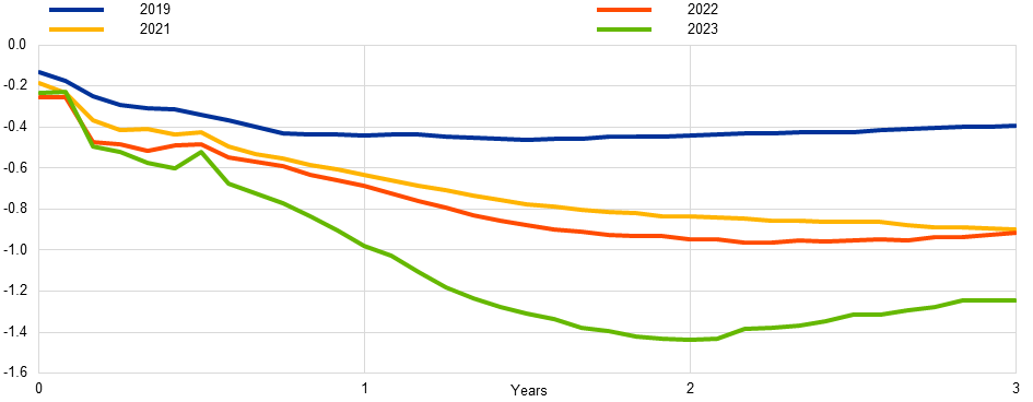
Beyond the baseline forecast
While the three-pronged reaction function of the Governing Council can be seen as an overarching strategy towards handling uncertainty about the economy and monetary transmission in the context of a major inflation shock and a significant monetary policy tightening cycle, staff also employ several techniques to identify and quantify the risks around the baseline projections. In this section, I will discuss some of these tools, but this should not be understood as an exhaustive list of the full set of sensitivity exercises that are run routinely at the ECB to chart out the range of plausible outcomes, conditional on the current state of information.
Indicators based on past projection errors
A good starting point is to use past forecast errors as a guide to quantifying uncertainty looking into the future, since projection errors can be interpreted as a catch-all proxy of all of the different sources of past uncertainty. At the ECB, these forecast errors are used to create fan charts based on ranges, with the width of such intervals calibrated to be twice the mean absolute value of past errors, excluding outliers.[23] The distribution is assumed to be perfectly symmetric, so no information is provided on the balance of risks. Uncertainty is illustrated through three different ranges, representing prediction intervals of 30%, 60% and 90%. These intervals indicate the probability that future observations will fall within these ranges if the typical shocks from the past, excluding exceptional events, were to occur again in the future. Knightian uncertainty is, therefore, ruled out by assumption.
A fan chart is a simple way to visualise, interpret and communicate forecast uncertainty based on past projection errors (Chart 7). It is a useful instrument for conveying complex information both to the Governing Council and in external communication. However, their construction based on historical data may lead to an incomplete picture of future uncertainties, especially in the face of atypical, asymmetric and outsized risks. In addition, fan charts do not explain which risks might affect the economy or the underlying mechanisms governing how the risks may travel through the economy. This lack of a narrative can leave policymakers without crucial insights into the underlying drivers of uncertainty about the inflation and growth outlook.
Chart 7
Euro area HICP inflation: baseline and projection error-based fan chart
(quarter-on-quarter percentage changes, seasonally and working day-adjusted quarterly data)
Sources: ECB calculations. Notes: The vertical line indicates the start of the current projection horizon. Inflation before this vertical line indicates data. The horizontal line indicates the 2% inflation target. The ranges shown around the central projections provide a measure of the degree of uncertainty and are symmetric by construction. The ranges are based on past projection errors, after adjustment for outliers. The bands, from darkest to lightest, depict the 30%, 60% and 90% probabilities that the outcome of HICP inflation will fall within the respective intervals.
Subjective probability distributions
Another method traditionally employed at the ECB to quantify forecast uncertainty is the application of subjective probability distributions. In each forecasting round, a survey is conducted among senior staff, which yields subjective probability distributions around the inflation and growth projections based on methods to aggregate their individual opinions into a collective judgement.[24] These experts also rank the risks and uncertainties that they consider to be most important, with the results reported to the Governing Council in a structured manner and discussed in the context of the risk outlook. This approach is transparent and easy to interpret for the Governing Council. It is also forward-looking and linked to tangible risks currently on the minds of staff, allowing us to anticipate different environments that may materialise in the future and understand which risks might be driving the distribution. At the same time, there is inherent subjectivity in this process, which means that the associated probability distributions are not entirely derived from empirical data. In addition, while individual risks are ranked, the specific mechanisms through which those risks could affect the economy remain unclear.
Model-based risk analysis
A model-based approach to quantifying macroeconomic risks is attractive, since it allows us to examine how current developments steer the entire distribution of future macroeconomic outcomes. This approach is inspired by a growing body of literature known as ‘macro-at-risk’.[25] At the ECB, staff have developed various macro-at-risk models to explore the way specific indicators influence the tail risks surrounding future real GDP growth and inflation.
One example is given by inflation-at-risk models that help us assess the potential risks to our inflation projections by estimating the probability distribution of future inflation outcomes at different points in time. The September projections indicated small downside risks to the 2024 HICP projections, although over a longer horizon such inflation-at-risk models still identified non-negligible upside risks (Chart 8).
Chart 8
Probability distributions of HICP inflation projections for 2025 based on inflation-at-risk models
(annual percentage changes)
Sources: ECB calculations. Notes: The chart depicts the predictive distributions of headline HICP inflation for the year 2025 from a combination of best-performing inflation-at-risk models. The combined density follows the quantile aggregation approach weighting the individual densities based on their corresponding (inverse of) average continuous ranked probability score. All distributions are assumed to follow skew-t distributions whose modes are tilted towards the September 2024 baseline projections. 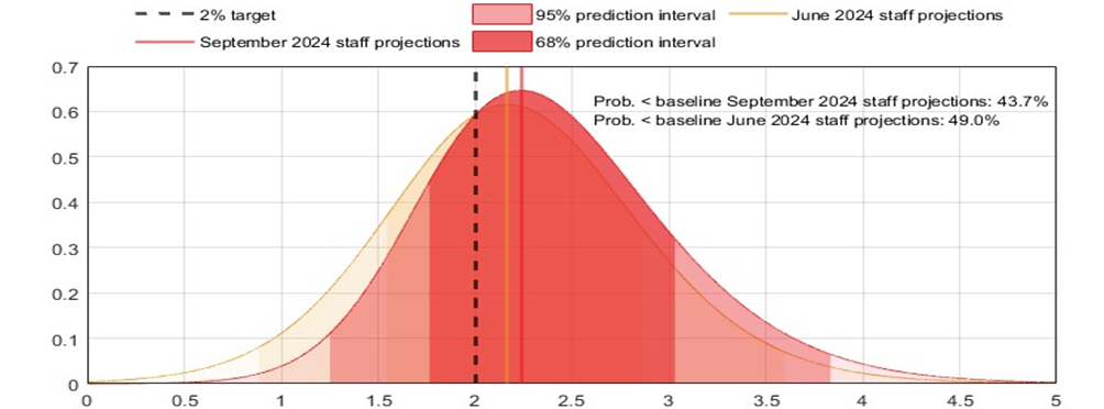
Another example of a macro-at-risk approach generates a path for the tails of the distributions for future macroeconomic variables by conditioning on monetary and financial developments. The resulting model-based estimates indicate that both upside and downside risks to growth in the coming years are consistent with historical patterns (Chart 9, left panel).
It is also possible to extract insights from the joint distribution of inflation and GDP. Recent exercises have indicated that, by end-2026, the probability of inflation undershooting the target is now greater than the probability of overshooting. High inflation realisations are more likely to occur in a context of subpar GDP growth, indicating that adverse supply shocks remain the primary source of upside risk to inflation (Chart 9, right panel).
Chart 9
Macro-at-risk model-based assessment of risk to euro area GDP growth and inflation
|
Paths of downside and upside tail risks for real GDP and inflation |
Joint growth- inflation risks |
|---|---|
|
(GDP: percentage deviation relative to 2024 Q2; inflation: year-on-year inflation, percentages) |
(probabilities in percentages) |
 |
 |
Sources: ECB and ECB calculations.
Notes: Left and centre panels: for each model, the paths are ranked based on the cumulative output (for GDP) and average inflation (for inflation) over the next 12 quarters. To get the downside (upside) paths, paths that fall between the 9th and 11th (89th and 91st) quantile of the relevant distribution are selected and averaged model by model. The panels present the average paths across the models, and two standard deviations of the path distribution computed across models as model uncertainty. Historical paths are computed by applying the same procedure to historical data for GDP and by selecting the relevant percentiles of the distribution for inflation.
Right panel: GDP around potential output is defined as within 0.5 percentage points of potential output. Grey bars denote the unconditional inflation distribution between the first quarter of 1999 and the fourth quarter of 2023. The latest observations are for the second quarter of 2024.
Sensitivity analysis related to market-based conditioning assumptions
Conditioning assumptions for the future evolution of key input variables are an important component of the ECB and Eurosystem staff projections. For example, the paths for inputs such as commodity prices, including oil and gas prices, are based on market expectations at the time of the projection cut-off date. Since market expectations are themselves variable (as markets continuously reassess the likely path of commodity valuations in response to news), staff systematically quantify the sensitivity of our baseline to changes in these assumptions.
For oil and gas prices, alternative paths are derived using percentiles of option-implied neutral densities, while staff additionally consider a constant-price assumption. We can illustrate this approach taking our September projections as the point of departure. At that time, oil prices were close to symmetrically distributed around the baseline assumption, indicating broadly balanced risks (Chart 10). However, the gas price distribution highlighted upside risks, probably reflecting adverse geopolitical developments such as escalating tensions in the Middle East and the incursion of Ukrainian troops into Russian territory. Staff modelled the effects on our projections of assuming the 25th percentile of these distributions, the 75th percentile, and constant prices. The findings from the September exercise indicated an upside skew to inflation risks but limited, balanced risks for GDP growth from the possible alternative paths for energy prices (Table 1).
Chart 10
Alternative paths for energy price assumptions
(USD/barrel for the oil price; EUR/MWh for the gas price
Sources: Morningstar and ECB calculations. Notes: Options-implied densities of gas and oil prices are extracted from 16 August 2024 market quotes of options on ICE Brent Crude Oil and Dutch TTF Natural gas futures with fixed quarterly expiry dates. The technical assumption refers to the paths of commodity prices implied by futures markets in the ten working days ending on the cut-off date, which was 16 August 2024 for the September projections.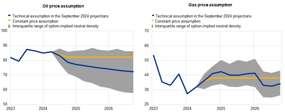
These sensitivity analyses are performed on different assumptions for market prices and are easy to interpret and communicate. These are also forward-looking in that they take account of current market conditions and expectations, providing a more relevant assessment of future risks stemming from the variables in focus than approaches based purely on past projection errors. However, market-based sensitivity analyses can only quantify risks from a limited subset of factors. And while these offer statistical insights, these do not condition on the fundamental forces driving a given shift in market prices.
Table 1
Effects of alternative energy price paths on real GDP growth and HICP inflation in the September 2024 projections
|
Path 1: 25th percentile |
Path 2: 75th percentile |
Path 3: constant prices |
|||||||
|---|---|---|---|---|---|---|---|---|---|
|
2024 |
2025 |
2026 |
2024 |
2025 |
2026 |
2024 |
2025 |
2026 |
|
|
(deviation from baseline levels, percentages) |
|||||||||
|
Oil prices |
-4.0 |
-14.1 |
-19.1 |
3.6 |
14.8 |
18.5 |
1.2 |
8.1 |
12.3 |
|
Gas prices |
-10.2 |
-19.8 |
-23.8 |
7.2 |
21.1 |
26.6 |
-2.4 |
-6.9 |
7.9 |
|
Synthetic energy price index |
-7.3 |
-16.8 |
-20.0 |
6.7 |
19.3 |
24.3 |
0.0 |
2.1 |
10.6 |
|
(deviations from baseline growth rates, percentage points) |
|||||||||
|
Real GDP growth |
0.0 |
0.1 |
0.1 |
0.1 |
-0.1 |
-0.1 |
0.0 |
0.0 |
0.0 |
|
HICP inflation |
-0.2 |
-0.6 |
-0.3 |
0.3 |
0.8 |
0.4 |
0.0 |
0.1 |
0.3 |
Notes: In this sensitivity analysis, a synthetic energy price index that combines oil and gas futures prices is used. The 25th and 75th percentiles refer to the option-implied neutral densities for the oil and gas prices on 16 August 2024. The constant oil and gas prices take the respective value as at the same date. The macroeconomic effects are reported as averages of a number of ECB and Eurosystem staff macroeconomic models.
This approach can also be augmented by using model-based density forecasts that do not just consider individual percentiles of option-implied densities but instead exploit the full distribution. This information can be incorporated into macroeconomic models using conditional density forecasting techniques. By imposing the forecasting density of one variable in the model, staff can explore how the densities of other variables react, with any asymmetric risks being inherited by the model. Chart 11 gives an example from the September projections exercise.[26] Options-implied energy price forecasting densities imply upside risks to inflation and downside risks to real economic activity, mainly towards the end of the projection horizon.
Model-based density forecasts can also be valuable in identifying and quantifying specific sources of projection uncertainty and anticipating future economic conditions, based on current market expectations. But these forecasts are not easy to communicate. The complexity of the models and the technical nature of the results can make it challenging to present insights clearly to policymakers. These forecasts also face model uncertainty and might struggle to capture the dynamics of future uncertainty, especially if there are structural changes in the economy. Finally, these can still only consider a limited subset of factors.
Chart 11
Conditional forecasts with option-implied densities
(annual percentage changes)
Sources: ECB staff calculations, based on the September 2024 projections baseline and Morningstar data. Notes: The chart shows model-based densities using a NAWM II version with an enhanced transmission of energy prices. The dashed blue lines show the 5% and 95% quantiles of the model-based densities centred around the baseline. The grey densities show the result of a conditional density forecasting exercise in which the forecasting densities of energy prices (oil and gas) are imposed to be those that come from options (see Montes-Galdón, C., Paredes, J., and Wolf, E. (2022), “Conditional Density Forecasting: A Tempered Importance Sampling Approach,” Working Paper Series, No. 2754, ECB). The densities show the 5%, 16%, 84% and 95% quantiles of the forecasting distributions. The transmission of energy prices in the model is enhanced by assuming a faster pass-through from energy prices to import prices. Oil and gas prices are drawn jointly to generate densities for the synthetic energy index with a correlation coefficient q=0.9 using Gaussian copulas.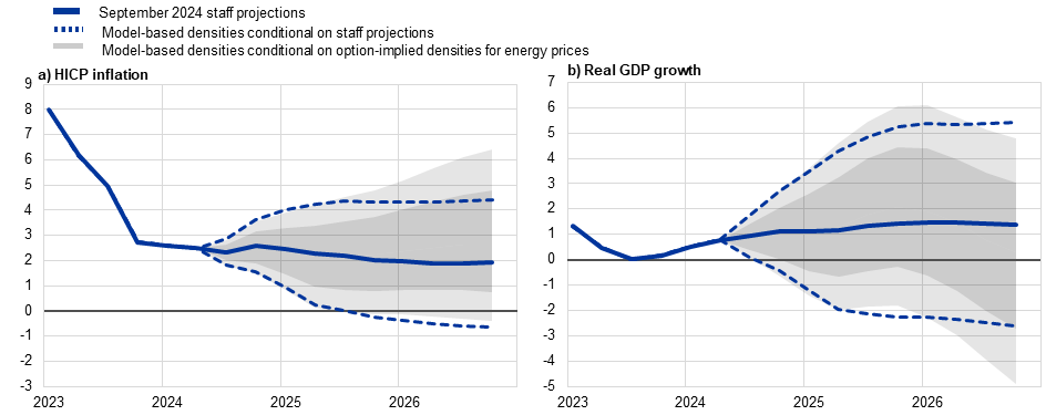
Scenario analysis
By tracing out the implications of a particular configuration of risks, scenario analysis provides another approach for communicating that the baseline is surrounded by a wide range of alternative future paths. Prior to the pandemic, staff conducted occasional scenario analysis, for example to model the implications of rare and unfamiliar occurrences, such as a no-deal Brexit. From March 2020 onwards, the ECB used this approach more intensively to navigate the turbulent waters of economic and geopolitical uncertainty. In each projection round, various scenarios of topical relevance are considered, with recent exercises covering, inter alia, an escalation of tensions in the Middle East and alternative scenarios for the evolution of labour productivity.
In some ways, scenario analysis is attractive in terms of interpretation and communication. It is particularly helpful in providing a narrative that explains how the crystallisation of a particular risk, or a constellation of inter-linked risks, might affect the economy. Scenario analysis is also naturally forward looking. It allows us to consider, and to some extent account for, various emerging challenges and potential future worlds. By focusing on the implications of particular scenarios even when it is very difficult to attach probabilities to their occurrence, it can also help to confront Knightian uncertainty.
At the same time, especially if not contextualised, an indiscriminate presentation of many scenarios might excessively shift the focus of attention away from the likeliest outcome towards hypothetical sets of circumstances that might only have a small probability of being realised. In the other direction, focusing on a too-small set of scenarios might divert attention from other looming risks.
One specific scenario analysis performed in the context of our September 2024 projections exercise was to explore the implications of potential shocks to consumer confidence.[27] This analysis used a semi-structural model to assess how unexpected changes in consumer confidence might affect household decisions on consumption, saving and housing investment. It then examined the broader implications for economic activity and inflation using a structural model.
Consumer confidence has been volatile since Russia’s invasion of Ukraine, and it has remained subdued despite some recent recovery (Chart 12). This scenario analysis explored three possibilities for the evolution of consumer confidence. A “lower confidence” scenario assumed that consumer confidence would deteriorate in the fourth quarter of 2024 and remain weak, likely due to increasing geopolitical uncertainty. When simulated through the model, this resulted in an increase in the saving ratio for precautionary reasons, also leading to a decline in housing investment. The “higher confidence” scenario reflected the polar case of improving confidence, likely related to rising real incomes. Finally, a “temporarily lower confidence” scenario assumed that the initial decline in consumer confidence would be followed by a rebound in the third quarter of 2025, so that the saving ratio would initially increase above the baseline but would later converge back to the baseline.
Chart 12
Private consumption, housing investment, the saving ratio and consumer confidence since 2022, and different scenarios for the evolution of consumer confidence
|
Private consumption, housing investment and the saving ratio |
Consumer confidence and uncertainty |
|---|---|
|
(left scale: annual percentage changes; right scale: share of gross disposable income, percentage) |
(standardised level) |
 |
 |
Sources: Eurostat, European Commission (Directorate General for Economic and Financial Affairs) and ECB staff calculations.
Notes: In the right panel, the data are standardised for the entire available sample – from January 1999 to August 2024 for confidence and from April 2019 to July 2024 for uncertainty. The dashed blue line refers to a projection of consumer confidence consistent with the baseline projections through the lens of an empirical model. In the right panel, the vertical line marks the start of the current projection horizon. The latest observations are for the first quarter of 2024 for the left panel and for August 2024 for the right panel. Scenario 1, “Lower confidence”, is constructed by imposing responses of housing investment and the saving ratio consistent with a positive one-standard-deviation shock to consumer confidence, while Scenario 2, “Higher confidence”, imposes the paths consistent with a negative one-standard-deviation shock. Scenario 3, “Temporarily lower confidence”, imposes the responses of housing investment and the saving ratio consistent with a negative one-standard-deviation shock followed by a positive shock of the same magnitude after four quarters.
The results indicated that, in the “lower confidence” scenario, real GDP growth would be 0.3 and 0.6 percentage points below the baseline in 2025 and 2026, respectively (Table 2). This scenario would also have a negative impact on private consumption and employment growth. In the “temporarily lower confidence” scenario, real GDP growth would see a cumulative deviation of -0.1 percentage points from the baseline over 2024-2026, with larger effects on private consumption. By contrast, GDP growth would be naturally above the baseline in the “higher confidence” scenario. In all scenarios there was only a very limited impact on the inflation outlook, due to the choice of shocks, which only directly have an impact on quantities, and a relatively flat Phillips curve in the model used for the scenario analysis,.
Table 2
Effects of consumer confidence scenarios on real GDP growth, HICP inflation and private consumption
(percentage point deviation from baseline)
|
Real GDP growth |
Private consumption growth |
HICP inflation |
||||||||||
|---|---|---|---|---|---|---|---|---|---|---|---|---|
|
2024 |
2025 |
2026 |
Cumulated |
2024 |
2025 |
2026 |
Cumulated |
2024 |
2025 |
2026 |
Cumulated |
|
|
Scenario 1: Lower confidence |
0.0 |
-0.3 |
-0.6 |
-0.9 |
0.0 |
-0.4 |
-0.9 |
-1.4 |
0.0 |
0.0 |
-0.1 |
-0.1 |
|
Scenario 2: Higher confidence |
0.0 |
0.3 |
0.5 |
0.9 |
0.0 |
0.4 |
0.9 |
1.4 |
0.0 |
0.0 |
0.1 |
0.1 |
|
Scenario 3: Temporarily lower confidence |
0.0 |
-0.3 |
0.1 |
-0.1 |
0.0 |
-0.4 |
0.1 |
-0.3 |
0.0 |
0.0 |
0.0 |
0.0 |
Sources: The ECB-BASE model and ECB staff calculations.
Notes: ECB-BASE simulation using the “projection update modality” with exogenous exchange rate and monetary and fiscal policies. Additionally, other channels that could amplify the effects of consumer confidence shocks, such as a corresponding international environment scenario or direct effects through expectations, are excluded. The response of private consumption is consistent with the ECB-BASE-implied response. All numbers are reported in percentage point deviations from the baseline and are rounded to one decimal place.
Calibration of monetary policy
The calibration of monetary policy is the next step the Governing Council needs to take after thoroughly analysing the risks and uncertainties surrounding the economy, as well as the strength of monetary transmission. Here, I will focus on a set of model-based policy simulations that are useful in informing our decision-making in an uncertain environment by exploring the potential outcomes of various policy actions, mainly over a short horizon. I will also say a few words about how risk management considerations have informed some of the recent policy decisions of the Governing Council.
Model-based policy simulations
Model-based policy simulations utilise a suite of structural or semi-structural macroeconomic models, the transmission channels of which represent state-of-the-art knowledge about the workings of the economy. These models allow us to implement different interest rate paths compared to the baseline market-based interest rate path that is embedded in the projections. This exercise lends robustness to our policy choices in the face of economic uncertainty and model uncertainty. As an illustration of this approach, I will revisit a policy exercise that staff conducted ahead of the June 2024 Governing Council.
The June projections were predicated on market expectations that entailed a cumulative 75 basis point cut in the deposit facility rate by the end of 2024. Policy simulations allowed us to assess three possible profiles that differed in the number of rate cuts by the end of 2024. All profiles assumed a 25 basis point cut in June 2024, which, by the time the exercise was conducted, was seen as highly likely by the market. The baseline (“intermediate”) profile implied two further 25 basis point cuts in the third and fourth quarters, resulting in a deposit facility rate of 3.25% by year-end, broadly in line with the market-based rate profile at the time. The most restrictive profile (“later”) implemented only a single further 25 basis point rate cut in the fourth quarter of 2024. The most accommodative (“earlier”) profile assumed a cumulative 50 basis point cut in Q3 2024, followed by another 25 basis point cut in Q4 2024.[28] All three scenarios were extended from the start of 2025 onwards along a trajectory dictated by an estimated reaction function that mapped the projected macroeconomic conditions into a rate response.
The implications of these alternative policy paths for inflation in 2024, 2025 and 2026 using three different models and based on the state of knowledge available in June 2024 are shown in Chart 13.[29] The most restrictive rate profile was effective in bringing inflation down to levels close to 2% in 2025, though with some dispersion of results across models. However, this rate profile could lead to a noticeable inflation undershoot in 2026. Conversely, the most accommodative profile was consistent with somewhat higher inflation in 2025. At a longer horizon, however, this policy trajectory would still deliver an inflation rate of 1.9%. Intuitively, because of its close alignment with the rate profile underlying the June projections, the intermediate profile was seen as delivering an outlook for inflation very close to the projection baseline.
Chart 13
Annual euro area inflation in the projections and under alternative policy paths based on information from June 2024
(annual percentage changes)
Sources: Eurosystem staff macroeconomic projections for the euro area, June 2024; ECB calculations using the New Area-Wide Model (Coenen, Karadi, Schmidt and Warne, 2019), the MMR model (Mazelis, Motto and Ristiniemi, 2023), and the BASE model (Angelini, Bokan, Christoffel, Ciccarelli and Zimic, 2019). Notes: Circles represent the annual inflation forecasts from the June 2024 projections. Ranges are constructed from the minimum and maximum of annual inflation rates across the three different models.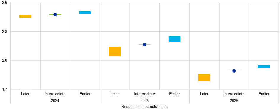
Beyond the central tendency of the staff projections and variations in the policy rate around the benchmark market curve, we also consider the performance of a range of possible interest rates paths under alternative macroeconomic forecasts. This supports robust policy making in the face of uncertainty and is particularly important during times of significant economic volatility. I will illustrate this robustness test in a stylised exercise.
Robust policy
A policy is defined as robust according to the min-max criterion, if it avoids the worst case scenario across a specified set of macroeconomic environments and policy tactics.[30] To illustrate this, let me describe an exercise in robust control where a structural model is used to simulate three environments: one based on the model’s estimated parameters; the second reflecting a worsening trade-off between inflation and output due to large supply shocks (“persistent inflation”); and the third increasing the role of demand shocks and increasing the impact of interest rates on the real economy to capture the unusual post-pandemic demand pressure and possibly amplified policy transmission.[31] Next, for each environment staff compute the associated optimal simple rule: the policy rule that maximises the policymaker’s objectives as defined by a loss function.[32] Then each of the optimal policy rules is deployed in each of the three environments and the losses are computed according to the stipulated loss function. Finally, policy performance is compared, as measured by these model-based loss calculations, across the different environments using a min-max strategy. Note that this approach abstracts from considering whether any particular environment is more or less likely to materialise than any other.
The first two environments are captured by the four cells in the top left corner of Table 3. A min-max strategy tries to avoid the outcome with the worst loss, which would be realised by following the baseline optimal policy (top row) in a “persistent inflation” environment (second column). Thus, a min-max approach suggests that, in the face of this particular source of uncertainty, it is advisable to generally implement a more forceful response to inflation, as indicated by the “persistent inflation” optimal policy (second row).
However, when considering all three environments (i.e. also including the third row and third column in Table 3), the largest loss arises when the “persistent inflation” policy (second row) is applied in the amplification environment (third column) and the baseline reaction is rather to be preferred from a min-max perspective.[33]
In summary, even a relatively simple model such as the one used to produce this exercise, can be helpful to policymakers in that it broadens their view of a whole range of possibilities – some expected, some undesirable – that may emerge as a result of their choices.
This highlights the value attached to broadening the information base on which the Governing Council takes decisions and systematically asking “what if” type of questions in the spirit of robust control to test our policy responses. In line with this insight, our meeting-by-meeting approach provides flexibility to respond nimbly to sudden shifts in the environment.
Table 3
Robust control
|
(percentage losses) |
|||||||||||||||||||||
|
|||||||||||||||||||||
Sources: ECB calculations using the MMR model with the exercises documented in the Handbook on Inflation (Coenen, Mazelis, Motto, Ristiniemi, Smets, Warne, Wouters (forthcoming)).
Notes: The persistent inflation environment is modelled via more persistent price mark-up shocks. The persistent risk premia and amplification effects environment is modelled via more persistent risk premium shocks and an amplification effect of policy on consumption, investment and more persistent risk premium shocks. Losses refer to the percentage increase in central bank losses relative to the baseline case. The loss function is given by ∑((πt-π* ) 2+λy y2 ) with πt measuring inflation, π* the inflation target, y ̃ the output gap, and the weight λy=0.2. The rows contain losses for policy rules that are chosen ex ante. The columns display the environments that materialise ex post. Each cell therefore displays the loss (in percent deviation from baseline) for a policy rule that was set based on expectations for the contingency presented in a row, while instead the contingency presented in the column materialises. The two cells with darker shades indicate the highest losses incurred under the persistent inflation environment and the amplification environment.
Risk management considerations have influenced some of the recent policy decisions of the Governing Council. For example, one motivation for the final interest rate hike in September 2023 was taking out insurance against a scenario in which the process of gradual disinflation that we were already observing at the time could stall or even reverse. The Governing Council came to the conclusion that it was safer to confront such a scenario with interest rates at 4% rather than 3.75%. An additional hike would reinforce progress towards our target for two basic reasons. First, if the economy evolved according to the staff baseline case, the decision to hike would bolster confidence that inflation will return to target within the projection horizon. Second, a higher interest rate would more strongly limit the amplification of any upside shocks to the inflation path. It followed that, all else equal, a more secure pace of disinflation and greater insurance against upside risks would also reinforce the anchoring of inflation expectations, which remained a precondition for the disinflation process to keep up its pace.
Precautionary risk management considerations also played an important role in motivating our latest monetary policy decision in October. If the slowdown signalled by recent economic activity indicators and the below target inflation print in September prove to be temporary, a decision to cut rates in October could, ex post, turn out as merely having brought forward a December cut. By contrast, if the recent data signalled a more persistent weakness, which confirms a stronger disinflationary process, cutting in October would, ex post, signal a nimble adjustment of policy to changing macroeconomic conditions. Retaining full optionality was therefore important and acted as a hedge against the materialisation of risks in either direction to the growth and inflation outlook. Communication should therefore continue to refrain from giving guidance about the speed and scale of monetary easing at future meetings.
Remaining open-minded about the speed and scale of adjustments is in fact a valuable strategy across various environments, as different situations may necessitate distinct approaches. Our confidence in a return of inflation to target has been growing for some time and, in response, we have gradually reduced our policy rates over the past months. This cautious approach, rooted in the principle of gradualism, emphasises moving incrementally when faced with uncertainty about the impact of our actions on the economy – after all, we cannot be certain that monetary transmission will retain its increased strength documented in the analysis presented earlier in this speech, or return to pre-pandemic elasticities.[34] This careful, step-by-step strategy enables us to observe the responses of the economy to our decisions and continuously refine our understanding of their impacts.
At the same time, gradualism is not a universal principle, as certain circumstances demand a more forceful response.[35] In fact, a prominent lesson can be drawn from our rate tightening measures at the onset of this policy cycle. After an initial phase when the persistence of the inflation surge was unclear and gradualism was one of our guiding principles, we swiftly moved out of negative territory and increased our policy rates in quick succession once it became clearer that persistence was indeed high, risking an upside de-anchoring of inflation expectations. Forceful rate actions (a pair of 75 basis point hikes in September and October 2022, followed by a triple of 50 basis points hikes between December 2022 and March 2023) were the appropriate response to avoid the risk that inflation expectations might de-anchor and, by dampening demand, to limit the scale and duration of second-round adjustments to the initial inflation shocks. Model-based estimates suggest that our decisive policy response reduced inflation rates by approximately two percentage points on average in each year between 2023 and 2026. Crucially, our rate decisions during this time helped to keep de-anchoring risks under control.[36]
Taken together, we are best served by making decisions in a state-dependent manner, taking into account the specific circumstances at hand. This flexible, meeting-by-meeting approach ensures that we remain responsive to the ever-changing economic landscape, enhancing our ability to effectively achieve our policy objectives.
Communication
To steer the economy through the current challenging times, a central bank needs to manage expectations – not only about inflation, but also about risks and uncertainties that can have major effects on our economy. By clearly conveying our economic outlook, risk assessment and policy decisions, we can help to reduce uncertainty and stabilise inflation expectations.
In this respect, as stressed in our 2021 Monetary Policy Strategy Statement, effective communication is a priority for us. In order to ensure that the message reaches its recipients and is well understood, we have been adjusting our language and expanding our communication channels. The monetary policy statement, published after each monetary policy meeting, is the principal channel through which the collective voice of the Governing Council reaches specialised economic observers and the public at large. The text needs to be made accessible to both constituencies. Indeed, the complexity of the statement, as measured by standard text analysis metrics, has decreased substantially (Chart 14). To further improve the understanding of our communication among non-technical audiences, we follow a layered approach, whereby the monetary policy statement is complemented by visual summaries laying out the essentials of our assessment about the economy and our policy choices.
Chart 14
Complexity of ECB monetary policy statements
(complexity score)
Source: Updated data (October 2024) from analysis in Coenen et al. (2017). Notes: The chart depicts the length and the complexity of the ECB’s monetary policy statements (known as the “introductory statement” until June 2021). The length is measured by the number of words (indicated by circle size). The difficulty of the language employed is measured using the Flesch-Kincaid Grade Level score, which indicates how many years of formal training are required to understand the text, based on the length of its sentences and words. Coenen et al. refers to Coenen, G., Ehrmann, M., Gaballo, G., Hoffmann, P., Nakov, A., Nardelli, S., Persson, E., and Strasser, G. (2017), “Communication of Monetary Policy in Unconventional Times,” Working Paper Series, No. 2080, ECB.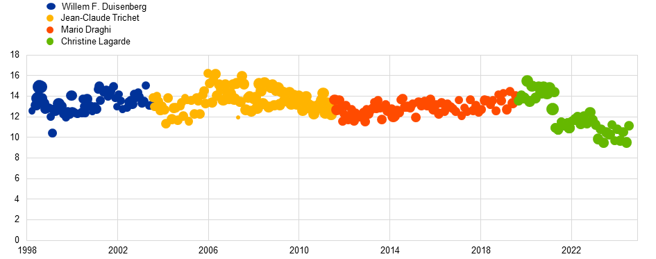
An important part of the monetary policy statement is the risk assessment section. This systematically highlights the Governing Council’s collective view on potential upside and downside risks to economic growth and inflation, drawing on the various factors analysed by staff using the methods and approaches discussed in this speech. As such, this section highlights particular uncertainties that the Governing Council identifies as surrounding the future outlook and provides some sense of how policy might need to be altered should different risks crystallise. Being transparent about alternative sets of circumstances that may push the economy onto trajectories that are different and possibly far from baseline does not mean necessarily being precise about the balance of those forces oftentimes pulling key macroeconomic variables in opposite directions.
Stressing state dependency and optionality, in line with the meeting-by-meeting and data-dependent approach, can help to avoid embracing a view or a policy approach, which could reduce our room for manoeuvre in conditions that we were unable to anticipate .[37] This ability to react flexibly is likely to be particularly useful when economic outcomes are dynamic and there is high uncertainty surrounding the outlook for inflation.
Conclusion
As I have laid out today, our monetary policy decisions are supported by a broad range of staff analyses on risks and contingencies, as well as through comprehensive simulations of monetary policy and stance scenarios. By effectively communicating our policy decisions and risk assessment, we enhance transparency and maintain public trust in our policy actions. And .it is essential that we are agile in responding to risks that might crystallise and new uncertainties that might emerge.
Our approach is not static. We are committed to the continuous development of our analytical toolkit, including by incorporating the latest research and advances from other policy institutions. Our 2025 assessment of our monetary policy strategy will provide an opportunity to reassess our current methods and explore new techniques and innovations. This will help us identify gaps or areas for improvement, ensuring that our toolkit remains comprehensive and state-of-the-art, allowing us to confront whatever forms of uncertainty we face in the coming years.
Finally, I want to conclude by differentiating between uncertainty about the macroeconomic cycle versus uncertainty about the economic trend. While I have been primarily focused on cyclical factors today, uncertainty about the trend also matters for monetary policy. In particular, the euro area economy could better withstand cyclical shocks if there were an improvement in the trend growth rate. To this end, the recommendations in the Letta and Draghi reports are of first order importance for the central bank, including a more ambitious agenda for capital markets union.[38]
คำแนะนำการอ่านบทความนี้ : บางบทความในเว็บไซต์ ใช้ระบบแปลภาษาอัตโนมัติ คำศัพท์เฉพาะบางคำอาจจะทำให้ไม่เข้าใจ สามารถเปลี่ยนภาษาเว็บไซต์เป็นภาษาอังกฤษ หรือปรับเปลี่ยนภาษาในการใช้งานเว็บไซต์ได้ตามที่ถนัด บทความของเรารองรับการใช้งานได้หลากหลายภาษา หากใช้ระบบแปลภาษาที่เว็บไซต์ยังไม่เข้าใจ สามารถศึกษาเพิ่มเติมโดยคลิกลิ้งค์ที่มาของบทความนี้ตามลิ้งค์ที่อยู่ด้านล่างนี้
Source link


